How many denoising steps does Boltz-1 need?
Protein structure prediction models following the AlphaFold 3 architecture involve three stages: input preparation (tokenization, retrieval e.g. of MSAs, embeddings), then a transformer-based representation learning “trunk”, and finally a diffusion-based structure module to predict structure. During inference, each denoising step runs one forward pass through the diffusion module, and the AlphaFold 3,1 Boltz-1,2 and Boltz-23 papers all used 200 sampling steps for prediction.
Recently there have been several works aiming to reduce the computational work of this sort of diffusion-based structure prediction process using flow maps - either distilled from a pretrained model4 or trained from scratch5.
Below are the results of some simple experiments which take the pretrained Boltz-1 model and look at:
- What the diffusion trajectories look like: the predicted denoised structure often arrives at the broad shape of the final prediction very early on, even after a single step.
- How much we can reduce the number of sampling steps without sacrificing prediction quality too much. This is a much simpler way to achieve more efficient inference than approaches that involve training new models.
- A comparison between outputs of the distogram head and the predicted structures, which suggests that the coarse geometry is often already present in the trunk representations before the diffusion module.
I chose to use Boltz-1 for these experiments because the evaluation code for Boltz-2 is not yet released. For experimentation I sampled a 50-target validation split from the released Boltz-1 test set, plus another 100 targets as a held-out test split. For details of the experimental setup, see appendix.
After running these experiments I came across Protenix-Mini6, which made a very similar observation for Protenix models: it is possible to dramatically reduce the number of sampling steps with very little impact on performance. This requires changes to the default AF3-style sampler; see their Section 3.1 and my appendix for more details.
Visualising 200-step trajectories
→ Open the animated trajectory viewer
This viewer shows denoising trajectories for two types of atom coordinates:
x0_pred, the predicted denoised coordinates (atom_coords_denoised in Boltz code)
and x_t, the post-update coordinates (atom_coords_next in Boltz code).
Looking at x0_pred, the rough shape of the structure often appears very early, even after the first denoising step.
(Some counterexamples:
8iha,
8tp8.)
Here are some plots which look at the x0_pred structure throughout the diffusion trajectories and compare it to A) the final prediction, B) the ground truth structure:

We see that predictions gradually get more similar to the final prediction (no surprise), but predictions after a single step are often already quite close to the final prediction.
There is not much improvement in RMSD against ground truth (sometimes it even gets worse over the trajectory).
This is consistent with the broad shape of the structure being decided early on.
However, the early x0_preds are not plausible structure predictions.
Looking at the first frame of an x0_pred trajectory shows implausible atom placements (e.g. 8agr sample 4, even though after just 1 step the RMSD to ground truth is ~1Å).
The local atom geometry takes some time to be resolved7.
Sweep over the number of sampling steps
Given that we’ve seen x0_pred reaches the rough shape of the final prediction pretty fast,
can we get the final prediction more efficiently by changing the sampling approach?
The simplest change is just to use fewer steps, though there are various other tricks one could try.
I ran a sweep over the number of denoising steps, trying {100, 50, 25, 20, 15, 10, 5} steps in comparison with the 200-step baseline.
I used Boltz’s default noise schedule, which is a Karras-style schedule8 with sigma_min=0.0004, sigma_max=160.0, sigma_data=16.0, and rho=8.
Here’s what the noise schedules look like for these:

Here are the results, looking at whether there is a degradation in the prediction quality metrics:

We see that 100 steps shows no degradation at all. 50, 25, and 20 steps are a bit ambiguous with some metrics showing positive changes and some negative, but all very small in magnitude and not statistically significant. 15 steps shows a small but statistically significant degradation in lDDT, but no degradations in RMSD, TM-score, or DockQ.
Decreasing to 10 and 5 steps results in a catastrophic degradation.
I later found out that this is largely due to step_scale=1.638 being set higher than 1 and setting step_scale=1 helps.
Scarpellini et al.4 apply this same fix for their Boltz-1x baselines when using diffusion steps.
See appendix for further details on this issue.
Further reducing the number of steps
The 15-step experiment uses the same Karras noise schedule parameters as the 200-step baseline, just with many fewer steps. However, there is no reason we need to stick to this functional form, or to expect that it is well-suited to the task of structure prediction.
When sampling from a trained diffusion model, […] we need to choose how to space things out as we traverse the different noise levels from high to low. In a range of noise levels that is more important, we’ll want to spend more time evaluating the model, and therefore space the noise levels closer together.
Sander Dieleman, “Noise schedules considered harmful”
To try to bring the number of steps below 15 without further degrading performance, I tested five modifications of the 15-step schedule, each compressing a different block of three steps into one (each of these schedules therefore takes 13 steps). Here are the results compared to the 15-step schedule as a baseline:

There is almost no impact in compressing the first three steps. There is very little impact in compressing the last three steps on RMSD, TM-score, or DockQ, but there is a large and statistically significant drop in lDDT - perhaps the last steps are performing local refinements that lDDT is more sensitive to.
Since compressing the first three steps had almost no effect, and since looking at a trajectory of , the initial noise levels seem extremely high, I tried simply starting from a lower initial noise. I used the level reached after 3 steps in the 15-step schedule, , resulting in a 12-step schedule. This showed almost no degradation compared to the 15-step schedule.
I then tried two further tweaks to this 12-step schedule starting from lower initial noise:
- Turn off churn (noise injection)
- In addition to turning off churn, set
step_scaleto 1 (default is 1.638)
I tried these after seeing something strange in the trajectory of x_t in the 15-step schedules: after a single step, x_t is already fairly close to the
rough shape of the final prediction, then the second and third steps increase the noise a lot.
At first I thought this was due to churn (hence variant 1) but it is actually caused by
step_scale=1.638, the same issue as mentioned above.
Briefly, at each step, the update is of the form
atom_coords_next = (1 - b) * (atom_coords + eps) + b * atom_coords_denoised
for some scalar coefficient b, which can become greater than 1 when step_scale > 1.
More details in the appendix.
Setting step_scale=1 fixes this “overshoot” issue so I tried applying this to the 12-step schedule to see if performance increases - unfortunately it degraded performance substantially in all metrics.
Here’s a summary of the accuracy of these candidate short schedules compared to the 200-step baseline:

Focussing on the 12-step schedule starting from lower initial noise, here are some more detailed comparisons between the 12-step schedule and the 200-step baseline:


12 steps vs 200 steps on held-out test set
I picked the 12-step schedule from a lower initial noise to evaluate on a test set consisting of 100 targets, a stratified sample of the Boltz-1 test set (see appendix for details) which was held out during the above iteration on schedules.

| Metric | Baseline | 12-step | Diff | 95% CI for Diff |
|---|---|---|---|---|
| lDDT | 0.7736 | 0.7539 | -0.0197 | [-0.0321, -0.0094] |
| RMSD | 8.2123 | 8.1940 | 0.0182 | [-0.2437, 0.2616] |
| TM-score | 0.8106 | 0.8075 | -0.0030 | [-0.0082, 0.0016] |
| DockQ | 0.2516 | 0.2518 | 0.0002 | [-0.0053, 0.0053] |

Open the held-out per-target plot.
The coarse structure is often already visible before the structure module
A distogram is a histogram, or binned probability distribution, of pairwise distances.
Boltz-1 has a distogram head which sits after the trunk and before the diffusion-based structure module. The distogram head simply symmetrises the pair representation across token pairs, then applies a linear projection from pair-channel dimension to distance-bin logits (Boltz-1 code). The outputs are logits for a distogram of pairwise distances between tokens, not atoms.
The distogram is used in Boltz-1 in two ways: it feeds directly into the loss function for training, and its outputs are also passed into the confidence module. It isn’t used to produce the structure prediction during inference.
I wanted to see if distogram predictions match up with the predicted structures output by the structure module. To compare a distogram with a predicted structure, I compute pairwise distances between the representative atoms in the predicted structure for each token. The distogram is a distribution over distances so I take a crude approach and for each token pair, pick the modal bin, and ask whether the corresponding distance in the predicted structure is in the modal bin, or close to it.
This was done using the default schedule with 200 sampling steps. Here are the results:

The four targets with the worst ±1 Å match rate are all quite complicated, and the Boltz-1 predictions are not close to the reference structures:
| PDB identifier | Diffusion trajectory | Description | Token-pair match rate at ±1 Å | Mean lDDT of predicted structures against ground truth |
|---|---|---|---|---|
| 8iks | Link | 16 short protein/peptide chains | 68.9% | 0.110 |
| 8psn | Link | 3 protein chains, 2 RNA chains, 3 Zn ions, 2 Mg ions | 82.2% | 0.197 |
| 8d4b | Link | 1 protein chain, 2 RNA chains | 92.6% | 0.559 |
| 8d4a | Link | 1 protein chain, 2 RNA chains, 2 DNA chains, 1 Zn ion, 2 Mg ions | 93.1% | 0.556 |
The match-rate numbers are a little hard to interpret on their own, so here are three examples in more detail showing the targets with the lowest, median, and highest ±1 Å match rate:
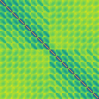
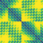
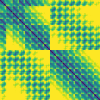
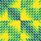
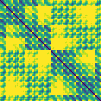
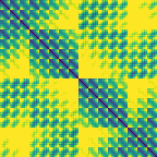

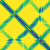

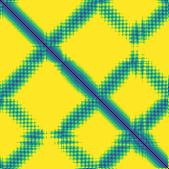
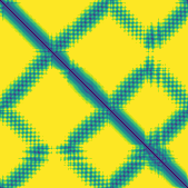

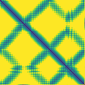
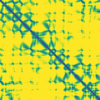
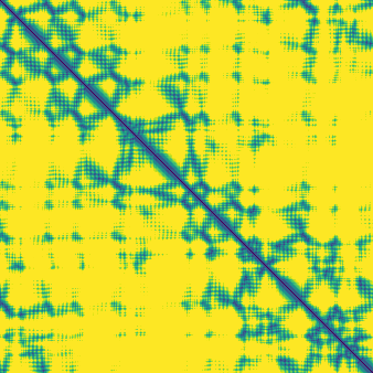

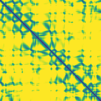
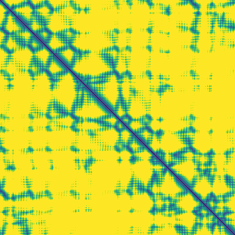

The comparisons here are between token-pair distograms and distances between corresponding representative atoms. The structure module does useful work in resolving the structure for all atoms and embedding this in 3D space. However, for the majority of these 50 structures, the distogram head outputs closely match the pairwise distances between representative atoms in the predicted structures. This raises the question of whether the diffusion module plays much of a role at all in determining the broad shape of the structure, or if this is generally already “decided” by the end of the trunk.
Discussion
Bearing in mind that these experiments use a small number of targets, I think these results point towards the following conclusions:
- The number of diffusion steps for Boltz-1 can be decreased substantially from 200 without harming performance. The 12-step schedule we evaluated on the test set did show a statistically significant degradation in average lDDT, although the degradation is not that large in magnitude. Looking at the detailed results, it’s a small number of targets which suffer from large degradations in quality.
- Denoising through the high-noise part of the schedule in particular doesn’t add value.
- The coarse geometry is often already present before diffusion (see the similarity between trunk distogram outputs and final predicted structures).
The final point makes me wonder how much the structure module is genuinely deciding the structure, versus just realising it in 3D.
I think changes to sampling are an attractive way to improve efficiency because they are simple to try, requiring no changes to the pretrained model.
Related work
The closest related work I’m aware of is Protenix-Mini6, which speeds up Protenix models in three ways,
including using a 2-step sampler for inference.
To get this to work they change the sampler to set step_scale=1 and gamma_0=0, i.e. no churn.
See Figure 4 of their paper for some results on a small-scale Protenix model.
They hypothesised that these trends would generalise to other AF3-style models.
I didn’t try 2-step inference but I did try 5- and 10-step schedules with step_scale=1 and the Boltz-1 default gamma_0=0.605 (results in appendix)
which perform reasonably well.
Another work which tried few-step sampling for Protenix is DCFold9. As a baseline for their distilled single-step model they run the pretrained model with a single sampling step (and also only one recycling step), also setting the step size to 1 and turning off churn - see their Section 4.1 / “AF3 ODE”.
The observation that the highest noise parts of the noise schedule don’t add much value at inference time was also made by Candido et al. for the ESMFold2 model10. ESMFold2 is a protein complex prediction model which uses representations from hidden layers of a pretrained protein language model, ESM-C, processed using recurrent folding layers, and finally an all-atom diffusion module. At inference, they use a schedule with 68 diffusion steps which is “truncated” from a 100 step schedule by starting from a lower initial noise (). See Section A.2.6 of the paper for their discussion.
Scarpellini et al.4 train flow map models distilled from Boltz-1 and Genesis’s proprietary Pearl model, to achieve few-step inference, supporting steering. Their Appendix C.1, Fig. 6 reports a comparison between their sampler and standard Boltz-1 sampling without steering, which is therefore comparable with my experiments. Their DECAF flow map method slightly beats standard Boltz-1 sampling at 5, 10, and 20 steps, with DECAF at 20 steps matching Boltz-1 at 200 steps, on the PoseBusters benchmark.
Finally, Kim11 examines the denoising trajectories of AlphaFold 3 and Boltz-2 using sparse autoencoders.
Thanks to Rishabh Anand for feedback on a draft.
Appendices
Experimental setup
I used the Boltz-1 PDB test set from this Google Drive link.
I modified boltz-community to:
- save detailed logs throughout the diffusion trajectory
- support arbitrary noise schedules
- support caching of the post-trunk tensors to make experiments on the structure module slightly cheaper to run.
For each denoising step I logged:
- schedule values:
sigma_tm,sigma_t,gamma, andt_hat - coordinates before the sampler update,
x_before_update - coordinates after adding churn noise,
x_noisy - the network’s denoised prediction,
x0_pred - coordinates after update,
x_t - atom padding mask,
atom_mask - masked token summary norms for
token_aandtoken_repr
I disabled Boltz’s default reordering of outputs by confidence.
Inference used Boltz-1 with recycling_steps=10, diffusion_samples=5, max_parallel_samples=5, --seed 1, and mmCIF output. Runs were on A100-80GB GPUs.
From the 542 released Boltz-1 PDB test examples, I sampled a 50-target validation split and a separate 100-target held-out test split, leaving 392 targets unused. I kept the number of examples so low because of a limited compute budget.
Stratification used StratifiedShuffleSplit(seed=1) over length_bucket, is_single_chain_input, and input_composition.
length_bucket:
short_<300: total polymer length < 300medium_300_700: 300 <= total polymer length <= 700long_>700: total polymer length > 700
total_length is the sum of sequence lengths over polymer entities only: protein, DNA, and RNA. If an entity has multiple chain IDs, its length is multiplied by the number of chain IDs. Ligands do not contribute to total_length.
is_single_chain_input is true if the input query has exactly one polymer chain ID, and false otherwise. Chain IDs came from each entity’s id field.
input_composition:
protein_only: kinds exactly{protein}protein_ligand: has protein and ligand, no nucleic acidprotein_nucleic: has protein and DNA/RNA, no ligandmixed_other: everything else, e.g. protein + ligand + nucleic acid, or other odd mixtures
Counts:
| Length bucket | Single-chain input | Input composition | Boltz-1 test set (n=542) | Validation (n=50) | Held-out test (n=100) |
|---|---|---|---|---|---|
| short | true | protein only | 55 | 5 | 10 |
| short | false | protein only | 40 | 4 | 7 |
| short | false | protein + ligand | 49 | 4 | 9 |
| short | false | protein + nucleic acid | 12 | 1 | 2 |
| short | false | mixed other | 8 | 1 | 2 |
| medium | true | protein only | 43 | 4 | 8 |
| medium | false | protein only | 66 | 6 | 12 |
| medium | false | protein + ligand | 106 | 10 | 20 |
| medium | false | protein + nucleic acid | 17 | 2 | 3 |
| medium | false | mixed other | 6 | 0 | 1 |
| long | true | protein only | 2 | 0 | 0 |
| long | false | protein only | 37 | 3 | 7 |
| long | false | protein + ligand | 43 | 4 | 8 |
| long | false | protein + nucleic acid | 19 | 2 | 4 |
| long | false | mixed other | 39 | 4 | 7 |
Final structures were evaluated with OpenStructure, using the same structure-evaluation flags as the released Boltz-1 evaluation script. I ran --patch-scores as a separate OpenStructure call because it sometimes failed even when the main structure metrics had succeeded. None of the results in this post use patch-score metrics, so this split only matters for keeping the core metrics rather than losing an otherwise usable evaluation.
The main structure metrics were produced with:
ost compare-structures \
  -m <prediction.cif> \
  -r <reference.cif[.gz]> \
  --fault-tolerant \
  --min-pep-length 4 \
  --min-nuc-length 4 \
  -o <structure_out.json> \
  --lddt \
  --bb-lddt \
  --qs-score \
  --dockq \
  --ics \
  --ips \
  --rigid-scores \
  --tm-score
The RMSD score computed is Cα/C3’ RMSD. For more details see
OpenStructure --rigid-scores documentation.
Coordinate tensors such as x0_pred and x_t are saved with padding, so I apply atom_mask before analysing them or writing structure files.
Overshooting x0_pred in sampler updates
The update to produce atom_coords_next, which I call x_t, in the Boltz code is (pseudocode):
atom_coords_next =
  atom_coords_noisy
+ step_scale * (sigma_t - t_hat) * (atom_coords_noisy - atom_coords_denoised) / t_hat
Letting b = step_scale * (1 - sigma_t / t_hat),
atom_coords_next = (1 - b) * atom_coords_noisy + b * atom_coords_denoised
Note: atom_coords_denoised is what I refer to as x0_pred,
and atom_coords_noisy = atom_coords + eps where eps is the noise added due to churn.
There is also a rigid alignment which I ignore.
If then the update is moving towards the denoised prediction atom_coords_denoised a.k.a. x0_pred.
If then the update is “overshooting” the denoised prediction.
is equivalent to sigma_t / t_hat < 1 - 1 / step_scale.
Now, t_hat = sigma_tm * (1 + gamma), where sigma_tm is the noise level we are moving from in the current step and sigma_t is the noise level we are moving to.
So, rearranging, is equivalent to:
sigma_t / sigma_tm < (step_scale - 1) * (1 + gamma) / step_scale
Therefore this never happens when step_scale = 1, but if step_scale > 1 it is possible, when the ratio sigma_t / sigma_tm between
the noise we are moving to and the noise we are moving from, is sufficiently small.
When the number of sampling steps is reduced to 15, the first update has and all subsequent updates are in the “overshoot” regime. This explains why the 15-step trajectories reach the rough shape of the final prediction after one step, then become noisier again in the next few steps.
I don’t see a clear reason why 15 steps still gives acceptable results but 10 steps does not.
However, I tried setting step_scale=1 for 5 and 10 step schedules (still with gamma=0.605)
and evaluating on the 50-target validation set, and the performance improved substantially:
| Schedule | Denoising calls | step_scale | lDDT | RMSD | TM-score | DockQ |
|---|---|---|---|---|---|---|
| 200-step baseline | 200 | 1.638 | 0.7880 | 7.6874 | 0.8003 | 0.2719 |
| 5-step | 5 | 1.638 | 0.0000 | 932.4256 | 0.0035 | 0.0000 |
| 5-step, step_scale=1 | 5 | 1 | 0.5179 | 7.6098 | 0.7963 | 0.2591 |
| 10-step | 10 | 1.638 | 0.0000 | 16.2630 | 0.4671 | 0.1005 |
| 10-step, step_scale=1 | 10 | 1 | 0.6948 | 7.5914 | 0.7975 | 0.2634 |
These results point in the same direction as results in Protenix-Mini6 (specifically Section 3.1), where they find that, for a small-scale Protenix model, changing the default AF3 sampler to use a step scale of 1 and no churn enables inference with as few as 1 or 2 steps without much drop in quality.
Footnotes
-
Josh Abramson, Jonas Adler, Jack Dunger, Richard Evans, Tim Green, Alexander Pritzel, Olaf Ronneberger, Lindsay Willmore, Andrew J. Ballard, Joshua Bambrick, et al., “Accurate structure prediction of biomolecular interactions with AlphaFold 3”, Nature 630, 493-500 (2024). ↩︎
-
Jeremy Wohlwend, Gabriele Corso, Saro Passaro, Noah Getz, Mateo Reveiz, Ken Leidal, Wojtek Swiderski, Liam Atkinson, Tally Portnoi, Itamar Chinn, et al., “Boltz-1: Democratizing Biomolecular Interaction Modeling”, bioRxiv (2025). ↩︎
-
Saro Passaro, Gabriele Corso, Jeremy Wohlwend, Mateo Reveiz, Stephan Thaler, Vignesh Ram Somnath, Noah Getz, Tally Portnoi, Julien Roy, Hannes Stark, et al., “Boltz-2: Towards accurate and efficient binding affinity prediction”, bioRxiv (2025). ↩︎
-
Gianluca Scarpellini, Ron Shprints, Peter Holderrieth, Juno Nam, Pranav Murugan, Rafael Gomez-Bombarelli, Tommi Jaakkola, Maruan Al-Shedivat, Nicholas Matthew Boffi, and Avishek Joey Bose, “Few-step Cofolding with All-Atom Flow Maps”, arXiv:2606.08375 (2026). ↩︎ ↩︎ ↩︎
-
Dongyeop Woo, Marta Skreta, Seonghyun Park, Kirill Neklyudov, and Sungsoo Ahn, “Riemannian MeanFlow”, arXiv:2602.07744 (2026). ↩︎
-
Chengyue Gong, Xinshi Chen, Yuxuan Zhang, Yuxuan Song, Hao Zhou, and Wenzhi Xiao, “Protenix-Mini: Efficient structure predictor via compact architecture, few-step diffusion and switchable PLM”, arXiv:2507.11839 (2025). ↩︎ ↩︎ ↩︎
-
In some rough initial experiments I saw that, on average, backbone lDDT was also quite high after just one step, while all-atom lDDT was very low initially and improved over the diffusion trajectory. ↩︎
-
Tero Karras, Miika Aittala, Timo Aila, and Samuli Laine: “Elucidating the design space of diffusion-based generative models”, Advances in Neural Information Processing Systems 35 (2022) ↩︎
-
Zhe Zhang, Yuanning Feng, Yuxuan Song, Keyue Qiu, Hao Zhou, and Wei-Ying Ma, “DCFold: Efficient protein structure generation with single forward pass”, arXiv:2605.17899 (2026). ↩︎
-
Salvatore Candido, Thomas Hayes, Alexander Derry, Roshan Rao, Zeming Lin, Robert Verkuil, Bryan Wu, Jin Sub Lee, Elise S. Bruguera, Jehan A. Keval, et al., “Language Modeling Materializes a World Model of Protein Biology”, preprint (2026). Code. ↩︎
-
Soo-Jeong Kim, “bish-bash-fold: what are protein structure prediction models learning?”, GenBio 2026 Spotlight. ↩︎